Introduction to gene expression programming
Gene expression programming (GEP) belongs to the family of evolutionary algorithms and is closely related to genetic algorithms and genetic programming (GP). Like GP, GEP is a special field of evolutionary computation that aims at building programs automatically to solve problems independently of their domain, i.e., the search space of GEP consists of computer problems and mathematical models. GEP was first developed by Cândida Ferreira in 2001 [1]. Over the past decades, GEP has attracted ever-increasing attention from the research communities, leading to a number of enhanced GEPs and applications proposed in the literature. A most recent review of GEP covering its further development and various applications is presented in [2].
The most significant difference between GEP and GP is that GEP adopts a linear fixed-length representation of computer programs, which can later be translated into an expression tree. By contrast, GP typically uses a variable-size syntax tree representation directly. DEAP has provided a gp module to support genetic programming. Many studies have claimed the superiority of GEP over the traditional GP in both efficiency and effectiveness.
Background of GEP
In this section, a short introduction of the GEP theory is presented to help users understand the terminology and the basic search mechanism in GEP.
Chromosome representation of GEP
In gene expression programming, the genome or chromosome consists of a linear, symbolic string of fixed length composed of one or more genes. Each gene itself is a fixed-length string composed of various primitives. Just following the terminology of GP, there are two kinds of primitives in GEP: function and terminal. A function is a primitive that can accepts one or more arguments and returns a result after evaluation, while a terminal represents a constant or a variable in a given program. In GEP, a gene is divided into two parts. The first part (called the head) is formed by functions and terminals, while the second part (called the tail) is formed by terminals only. An example of a gene of head length 5 and tail length 6 is given below, where the head part is colored in blue and the tail part is in green.
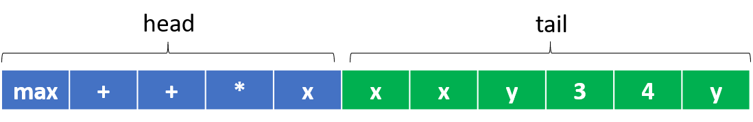
The above gene has three types of functions (max, +, *) and four terminals (x, y, 3, 4), where x and y are input variables. As we see, the head part is composed of four functions and one terminal, while the tail part is formed totally with terminals only, which is compulsory in GEP.
Genotype to phenotype translation
Given a fixed-length gene in GEP, as shown above, the expression of the genetic information is very simple. The genome is similar to level-order serialization of a syntax tree, which is called an expression tree (ET) in GEP. Specifically, in GEP starting from the first position of a gene, we can construct an expression tree through level-order traversal according to the arity of each function. (Arity is the number of arguments a function accepts.) The expression tree of the above gene is shown below (source ).
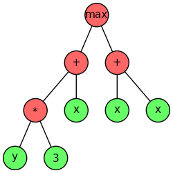
It is easy to notice that the last two elements in the gene don’t appear in the expression tree. Although in GEP the start site is always the first position of a gene, the termination point does not always coincide with the last position of a gene. It is common for GEP genes to have non-coding regions downstream of the termination point. In such a sense, the decoding of genes (or chromosomes) into expression trees is similar to gene expression in nature. The coding region of a gene is called open reading frames (ORFs), which is also named K-expression in GEP. Obviously, the ORF (K-expression) of the above gene is [max, +, +, *, x, x, x, y, 3], exactly the level-order traversal result of the corresponding expression tree.
As stated previously, GEP chromosomes have fixed length and are composed of one or more genes of equal length. Therefore the length of a gene is also fixed. Thus, in GEP, what varies is not the length of genes (which is constant), but the length of the ORFs. Indeed, the length of an ORF may be equal to or less than the length of the gene. Due to the possible existence of non-coding regions in GEP genes, a gene of a fixed length can encode a variety of expression trees, i.e., computer programs or mathematical expressions. To ensure the validness of a gene, for each problem, the length of the head h is chosen, whereas the tail length t is determined automatically by
where n is the maximum arity of all functions, i.e., the number of arguments of the function with the most arguments.
For example, given a function set \(F=\{Q, *, /, -, +\}\) (Q represents the square root), and a terminal set \(T=\{a, b\}\), supposing the head length of a gene is chosen to be \(h=10\). Then, since the maximum arity of the given functions is \(n=2\), the tail length is determined to be \(t = h(n - 1) + 1=11\). It is straightforward to see that no matter how a gene is composed, it always yields a valid expression tree, as long as it satisfies the length condition \(t = h(n - 1) + 1\). Some examples of genes and the associated expression trees after decoding are listed in the following (copied form [1], and the tail is shown in green).
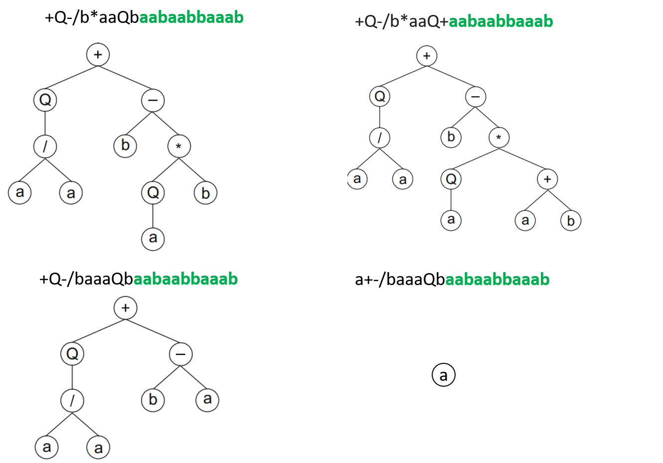
Pay special attention to the last expression tree in the above, where only a terminal node is expressed. Now it is clear that a gene of a fixed length can be translated into expression trees of various sizes.
Multigenic chromosomes
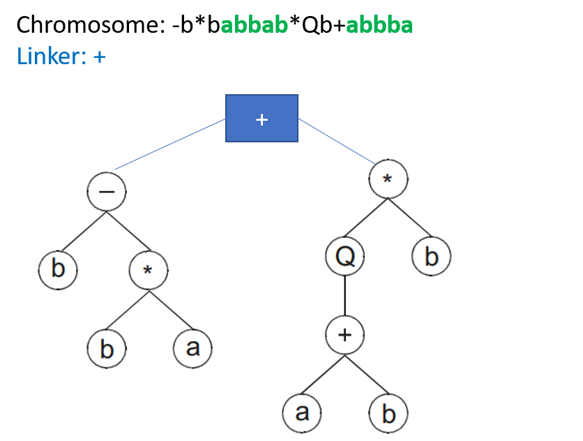
The individual concept in general evolutionary computation refers to an encoded solution of the given problem. In GEP, an individual is represented by a chromosome, which may contain one or more genes. A chromosome with only one gene is called a monogenic chromosome, whereas a chromosome composed of multiple genes is named a multigenic one. A multigenic chromosome is especially useful when solving complex problems by decomposing a complicated solution into several parts, each part encoded by a gene, for they permit the modular construction of complex, hierarchical structures. In a multigenic chromosome, each gene is translated into a sub-ET (expressed tree), and typically a linking function, or linker, is used to combine the sub-ETs into a single one. The following is an example of a chromosome composed of two genes, each gene of head length 4 and tail length 5, and the linking function is an addition.
The basic gene expression algorithm
Like all other evolutionary algorithms, GEP takes an initial population, and then evolves this population by selection, mutation and crossover, while the fitness of each individual is determined by a specific fitness evaluation function according to the problem definition. The only difference of GEP is that it has its own set of genetic operators specially designed to work with its linear, fixed-length and multigenic representation. The fundamental steps of the gene expression algorithm (GEA) are schematically represented below.
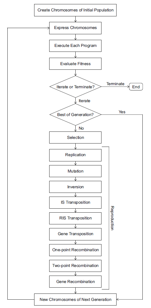
The above figure is taken from Cândida Ferreira’s monograph on GEP [3]. Some important components are explained as follows.
- The chromosome expression is supported by geppy, which compiles each GEP individual (chromosome) into an executable Python lambda expression and this program is subsequently evaluated with the user-defined fitness evaluation functions.
- The recommended selection methods are fitness-proportionate ones, such as the common roulette-wheel selection. However, other selection methods like tournament selection can also be used depending on specific problems.
- Mutation, inversion, and tranposition are all genetic operators which modify the genome of each individual.
- For crossover (mating), one-point and two-point recombination are both used. Besides, for multigenic chromosomes, a special crossover mechanism called gene recombination is also adopted.
- All the above modification and crossover happens with a custom probability.
GEP implementation in geppy
Data structures corresponding to the above terminology and concept in GEP are provided in geppy, for example, classes including Primitive, Function, Terminal, Gene, Chromosome, KExpression, etc. Besides, basic GEP algorithms are also built in the geppy.algorithms.basic module, which can avoid the boilerplate code for common tasks like symbolic regression.
For more details on how to implement GEP in geppy, please check the Overview of geppy for Gene Expression Programming (GEP) tutorial.
Reference
[1] Ferreira, C. (2001). Gene Expression Programming: a New Adaptive Algorithm for Solving Problems. Complex Systems, 13.
[2] Zhong, J., Feng, L., & Ong, Y. S. (2017). Gene expression programming: a survey. IEEE Computational Intelligence Magazine, 12(3), 54-72.
[3] Ferreira, C. (2006). Gene expression programming: mathematical modeling by an artificial intelligence (Vol. 21). Springer.